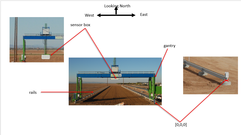
Geospatial information

Several different sensors include geospatial information in the dataset metadata describing the location of the sensor at the time of capture.

Coordinate reference systems The Scanalyzer system itself does not have a reliable GPS unit on the sensor box. There are 3 different coordinate systems that occur in the data:

Most common is EPSG:4326 (WGS84) USDA coordinates
Tractor planting & sensor data is in UTM Zone 12
Sensor position information is captured relative to the southeast corner of the Scanalyzer system in meters

EPSG:4326 coordinates for the four corners of the Scanalyzer system (bound by the rails above) are as follows:

NW: 33° 04.592' N, -111° 58.505' W
NE: 33° 04.591' N, -111° 58.487' W
SW: 33° 04.474' N, -111° 58.505' W
SE: 33° 04.470' N, -111° 58.485' W

In the trait database, this site is named the "MAC Field Scanner Field" and its bounding polygon is "POLYGON ((-111.9747967 33.0764953 358.682, -111.9747966 33.0745228 358.675, -111.9750963 33.074485715 358.62, -111.9750964 33.0764584 358.638, -111.9747967 33.0764953 358.682))"

Scanalyzer coordinates Finally, the Scanalyzer coordinate system is right-handed - the origin is in the SE corner, X increases going from south to north, and Y increases from east to the west.

In offset meter measurements from the southeast corner of the Scanalyzer system, the extent of possible motion for the sensor box is defined as:

NW: (207.3, 22.135, 5.5)
SE: (3.8, 0, 0)

Scanalyzer -> EPSG:4326 1. Calculate the UTM position of known SE corner point 2. Calculate the UTM position of the target point, using SE point as reference 3. Get EPSG:4326 position based on UTM

MAC coordinates Tractor planting data and tractor sensor data will use UTM Zone 12.

Scanalyzer -> MAC Given a Scanalyzer(x,y), the MAC(x,y) in UTM zone 12 is calculated using the linear transformation formula:

ay = 3659974.971; by = 1.0002; cy = 0.0078;
ax = 409012.2032; bx = 0.009; cx = - 0.9986;
Mx = ax + bx * Gx + cx * Gy
My = ay + by * Gx + cy * Gy

Assume Gx = -Gx', where Gx' is the Scanalyzer X coordinate.

MAC -> Scanalyzer

Gx = ( (My/cy - ay/cy) - (Mx/cx - ax/cx) ) / (by/cy - bx/cx)
Gy = ( (My/by - ay/by) - (Mx/bx - ax/bx) ) / (cy/by - cx/bx)

MAC -> EPSG:4326 USDA We do a linear shifting to convert MAC coordinates in to EPSG:4326 USDA

Latitude: Uy = My - 0.000015258894
Longitude: Ux = Mx + 0.000020308287

Sensors with geospatial metadata

stereoTop
flirIr
co2
cropCircle
PRI
scanner3dTop
NDVI
PS2
SWIR
VNIR

Available data All listed sensors

"gantry_system_variable_metadata": {
      "time": "08/17/2016 11:23:14",
      "position x [m]": "207.013",
      "position y [m]": "3.003",
      "position z [m]": "0.68",
      "speed x [m/s]": "0",
      "speed y [m/s]": "0.33",
      "speed z [m/s]": "0",
      "camera box light 1 is on": "True",
      "camera box light 2 is on": "True",
      "camera box light 3 is on": "True",
      "camera box light 4 is on": "True",
      "y end pos [m]": "22.135",
      "y set velocity [m/s]": "0.33",
      "y set acceleration [m/s^2]": "0.1",
      "y set decceleration [m/s^2]": "0.1"
    },

stereoTop

"sensor_fixed_metadata": {
      "cameras alignment": "cameras optical axis parallel to XAxis, perpendicular to ground",
      "optics focus setting (both)": "2.5m",
      "optics apperture setting (both)": "6.7",
      "location in gantry system": "camera box, facing ground",
      "location in camera box x [m]": "0.877",
      "location in camera box y [m]": "2.276",
      "location in camera box z [m]": "0.578",
      "field of view at 2m in X- Y- direction [m]": "[1.857 1.246]",
      "bounding Box [m]": "[1.857     1.246]",
    },

cropCircle

"sensor_fixed_metadata": {
      "location in gantry system": "camera box, facing ground",
      "location in camera box x [m]": "0.480",
      "location in camera box y [m]": "1.920",
      "location in camera box z [m]": "0.6",
    },

co2Sensor

"sensor_fixed_metadata": {
      "location in gantry system": "camera box, facing ground",
      "location in camera box x [m]": "0.35",
      "location in camera box y [m]": "2.62",
      "location in camera box z [m]": "0.7",
    },

flirIrCamera

"sensor_fixed_metadata": {
      "location in gantry system": "camera box, facing ground",
      "location in camera box x [m]": "0.877",
      "location in camera box y [m]": "1.361",
      "location in camera box z [m]": "0.520",
      "field of view x [m]": "1.496",
      "field of view y [m]": "1.105",
    },

ndviSensor

"sensor_fixed_metadata": {
      "location in gantry system": "top of gantry, facing up, camera box, facing ground",
      "location in camera box x [m]": "0.33",
      "location in camera box y [m]": "2.50",
    },

priSensor

"sensor_fixed_metadata": {
      "location in gantry system": "top of gantry, facing up, camera box, facing ground",
      "location in camera box x [m]": "0.400",
      "location in camera box y [m]": "2.470",
    },

SWIR

"sensor_fixed_metadata": {
      "location in gantry system": "camera box, facing ground",
      "location in camera box x [m]": "0.877",
      "location in camera box y [m]": "2.325",
      "location in camera box z [m]": "0.635",
      "field of view y [m]": "0.75",
      "optics focal length [mm]": "25",
      "optics focus apperture": "2.0",
    },

field scanner plots

There are 864 (54*16) plots in total and the plot layout is described in the plot plan table.

dimension	value
# rows	32
# rows / plot	2
# plots (2 rows ea)	864
# ranges	54
# columns	16
row width (m)	0.762
plot length (m)	4
row length (m)	3.5
alley length (m)	0.5

The boundary of each plot changes slightly each planting season. The scanalyzer coordinates of each row and each range of the two planting seasons is available in the field book. The scanalyzer coordinates of each plot are transformed into the (EPSG:4326) USDA coordinates using the equations above. After that, a polygon of each plot can be generated using ST_GeomFromText funtion and inserted into the BETYdb through SQL statements.

An Rcode is available for generating SQL statements based on the scanalyzer coordinates of each plot, which takes range.csv and row.csv as standard inputs.

The range.csv should be in the following format:

range	x_south	x_north
1	...	...
2	...	...
3	...	...
...	...	...

And the row.csv should look like:

row	y_west	y_east
1	...	...
2	...	...
3	...	...
...	...	...

The output will be something look like:

INSERT INTO sites (sitename, geometry) VALUES ( 'MAC Field Scanner Field Plot 1 Season 2',
ST_GeomFromText('POLYGON((-111.975049874375 33.0745312921391 353, -111.975033517034 33.0745313124814 353, 
-111.975033529346 33.0745670737771 353, -111.975049886694 33.0745670534346 353, -111.975049874375 
33.0745312921391 353))', 4326));

PreviousGenomics data NextHyperspectral imaging data

Last updated 5 years ago