Overview

This user manual is divided into the following sections:

• Data Products: A summary of the available data products and the processes used to create them

• Data Access: Instructions for how to access the data products using Clowder, Globus, BETYdb, and CoGe

• Description of the

• : Information about data use and attribution

• : In-depth examples of how to access and use the TERRA-REF data

What data is available?

• Raw output from sensors deployed on the Lemnatec field scanner

  • Additional data from greenhouse systems, UAVs, and tractors have not been released, but can be accessed through our beta user program

• Manually-collected fieldbooks and associated protocols

• Derived data, including phenomics data, from computational approaches

You can access genomics data in one of the following locations:

• Download via .

• The for download or use within the CyVerse computing environment.

• The computing environment.

Please review our .

The data is structured on both the TERRA-REF strorage (accessible via Globus and Workbench) and CyVerse Data Store infrastructures as follows:

The following table lists available TERRA-REF data products. The table will be updated as new datasets are released. Links are provided to pages with detailed information about each data product including sensor descriptions, algorithm (extractor) information, protocols, and data access instructions.

https://terraref.github.io/tutorials/accessing-trait-data-in-r.html

Several different sensors include geospatial information in the dataset metadata describing the location of the sensor at the time of capture.

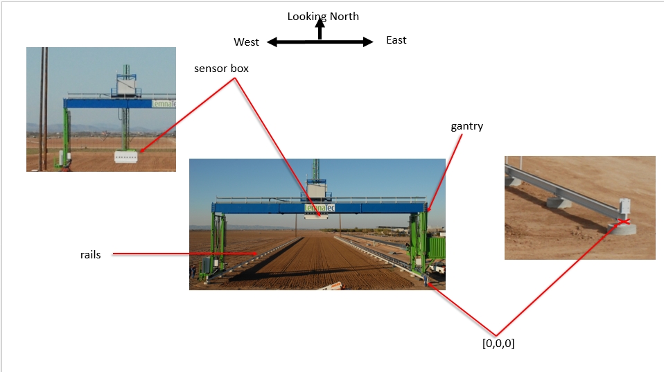
Coordinate reference systems The Scanalyzer system itself does not have a reliable GPS unit on the sensor box. There are 3 different coordinate systems that occur in the data:

• Most common is EPSG:4326 (WGS84) USDA coordinates

• Tractor planting & sensor data is in UTM Zone 12

• Sensor position information is captured relative to the southeast corner of the Scanalyzer system in meters

Summary

Infrared heat imaging data is collected collected using the FLIR SC615 thermal sensor. These data are provided as geotiff image raster files as well as plot level means.

• Algorithms are in the repository; see the readme for details.

Summary

3D point cloud data is collected using the Fraunhofer 3D laser scanner. Custom software installed at Maricopa converts .png output to the .ply point clouds. The .ply point clouds are converted to georeferenced .las files using the 3D point cloud extractor

Level 1 data products are provided in both .las and .ply formats. Raw sensor output (PLY) is converted to LAS format using the ply2las extractor; ply2las extractor code is available on GitHub.

For each scan, there are two .ply files representing two lasers, one on the left and the other on the right. These are combined in the .las files.

Sensor information

For details about using this data via Clowder or Globus, please see section.

Data access

Data is available via Clowder, Globus, and Workbench.

• Clowder:

• Globus or Workbench File System:

  • LAS /raw_data/laser3D_las

  • PLY /raw_data/laser3D

Known issues

• The position of the lasers is affected by temperature. We added a correction for temperature to adjust for this effect. See

Overview

TERRA-REF data can be accessed through many different interfaces: Globus, Clowder, BETYdb, CyVerse, and CoGe. Raw data is transfered to the primary compute pipeline using Globus Online. Data is ingested into Clowder to support exploratory analysis. The Clowder extractor system is used to transform the data and create derived data products, which are either available via Clowder or published to specialized services, such as BETYdb.

Public Domain Data

Data will be released with a CC0 license, meaning that they are in the public domain. The CC0 license allows wide use of these data and while it does not legally bind users to acknowledge the source data users are expected cite our data and research in publications, presentations, and other products.

The first release in 2020 included data from Seasons 4 and 6. This is available on Dryad and Globus.

Data are in the public domain to enable broad and unrestricted re-use. However, any derived pubications should cite the dataset:

Citing TERRA REF data:

Genomics, sensor, and phenotype data: LeBauer, David et al. (2020), Data From: TERRA-REF, An open reference data set from high resolution genomics, phenomics, and imaging sensors, Dryad, Dataset,

AZMet Weather Data (available on Dryad): Brown, P. W., and B. Russell. 1996. “AZMET, the Arizona Meteorological Network. Arizona Cooperative Extension.” .

Data Processing Pipeline: Burnette, Maxwell, et al. "TERRA-REF data processing infrastructure." Proceedings of the Practice and Experience on Advanced Research Computing. 2018. 1-7.

Software and Algorithms

For algorithms, we intend to release via BSD 3 clause or MIT / BSD compatible license. Algorithms are available on GitHub in the terraref organization: and have been archived on Zenodo (see ).

Citations for Individual Software and Documentation Components are listed in the section and can be browsed on .

Unpublished Data

We plan to make data from the Transportation Energy Resources from Renewable Agriculture Phenotyping Reference Platform (TERRA-REF) project available for use with attribution.

Please consider engaging with team members to collaborate on new research with these data. You can learn more about our approach to co-authorship and also about planned research papers in the section .

Timing of Future Data Releases

Any access to data prior to publication is granted with the understanding that the contributions and interests of the TERRA-REF team should be recognized and respected by the users of the data. The TERRA-REF team reserves the right to analyze and published its own data. Resource users should appropriately cite the source of the data and acknowledge the resource produces. The publication of the data, as suggested in the , should specify the collaborative nature of the project, and authorship is expected to include all those TERRA-REF team members contributing significantly to the work.

Planned future releases include Sorghum Season 9, data from experiments at Kansas State University, and data from the Danforth Indoor Phenotyping Facility.

Additional seasons can be requested as needed. We can provide the raw data and software required to process it. We can also collaborate with you to process the data, but this will typically require new funding sources.

Contacts

• Todd Mockler, Project/Genomics Lead (email: [email protected])

• David LeBauer, Computing Pipeline Lead (email: [email protected])

• Nadia Shakoor, Project Director (email: [email protected])

See also in the Introduction.

Summary

Fluorescence intensity data is collected using the PSII camera.

Each measurement produces 102 bin files. The first (index 0) is an image taken right before the LED are switched on (dark reference). Frame 1 to 100 are the 100 images taken, with the LEDs on. In binary file 102 (index 101) is a list with the timestamps of each frame of the 100 frames.

Right now the LED on timespan is 1s thus the first 50 frames are taken with LEDs on the latter 50 frames with LED off.

Raw data access

Fluorescence intensity data is available via Clowder and Globus:

• Clowder: __

• Globus paths:

  • /raw_data/ps2top

See also

Herritt, Matthew T., et al. "Chlorophyll fluorescence imaging captures photochemical efficiency of grain sorghum (Sorghum bicolor) in a field setting." Plant Methods 16.1 (2020): 1-13.

Environment conditions data is collected using the Vaisala CO2, Thies Clima weather sensors as well as lightning, irrigation, and weather data collected at the Maricopa site.

Data formats follow the Climate and Forecast (CF) conventions for variable names and units. Environmental data are stored in the Geostreams database.

Data sources

• WeatherStation coordinates are 33.074457 N, 111.975163 W

• EnvironmentLogger is on top of the gantry system and is moveable.

• Irrigation is managed at the field level. There are four regions that can be irrigated at different rates.

Data access

Level 1 data

Level 1 meteorological data is aggregated to from 1 Hz raw data to 5 minute averages or sums.

netCDF: 5s (12 per minute) observations

On Globus or Workbench you can find these data provided in both hourly and daily files. These files contain data at the original temporal resolution of 1/s. In addition, they contain the high resolution spectral radiometer data.

sites/ua-mac/Level_1/envlog_netcdf

• hourly files: YYYY-MM-DD_HH-MM-SS_environmentallogger.nc

• daily files: envlog_netcdf_L1_ua-mac_YYYY-MM-DD.nc

Geostreams: 5 minute observations

Data can be accessed using the geostreams API or the PEcAn meteorological workflow. These are illustrated in the .

Here is the json representation of a single five-minute observation:

Data can be accessed using the geostreams API or the PEcAn meteorological workflow.

These are illustrated in the .

Here is the json representation of a single five-minute observation from Geostreams:

Variable names and units

Raw Data

Data is available via Globus or Workbench:

• /ua-mac/raw_data/co2sensor

• /ua-mac/raw_data/EnvironmentLogger

• /ua-mac/raw_data/irrigation

• /ua-mac/raw_data/lightning

Sensor information:

Computational pipeline

• Description: EnvironmentalLogger raw files are converted to netCDF.

Known Issues

Known issue: the irrigation data stream does not currently handle variable irrigation rates within the field. Specifically, we have not yet accounted for the Summer 2017 drought experiments. See for more information.

When the full field is irrigated (as is typical), the irrigated area is 5466.1 m2 (=215.2 m x 25.4 m)

In 2017:

• Full field irrigated area from the start of the season to August 1 (103 dap) is 5466.1 m2 (=215.2 m x 25.4 m).

• Well-watered treatment zones from August 1 to 15 (103 to 116 dap): 2513.5 m2 (=215.2 m x 11.68 m) in total, combined areas of non-contiguous blocks

• Well-watered treatment zones from August 15 - 30 (116 to 131 dap): 3169.9 m2 (=215.2 m x 14.73 m), again in total as the combined areas of non-contiguous blocks

Github Issues

LemnaTec Scanalyzer 3D platform at the Donald Danforth Plant Science Center

Phenotype data is derived from images generated by the indoor LemnaTec Scanalyzer 3D platform at the Donald Danforth Plant Science Center using PlantCV. PlantCV is an image analysis package for plant phenotyping. PlantCV is composed of modular functions in order to be applicable to a variety of plant types and imaging systems. PlantCV contains base functions that are required to examine images from an excitation imaging fluorometer (PSII), visible spectrum camera (VIS), and near-infrared camera (NIR). PlantCV is a fully open source project: https://github.com/danforthcenter/plantcv. For more information, see:

Project website: http://plantcv.danforthcenter.org

Full documentation:

Publications:

To learn more about PlantCV, you can find examples in the repository, which is accessible on GitHub and in the TERRA REF under tutorials/plantcv

• an ipython notebook demonstration of PlantCV .

For the TERRA-REF project, a PlantCV Clowder extractor was developed to analyze data from the at the Donald Danforth Plant Science Center. Resulting phenotype data is stored in BETYdb.

Computational pipeline

• Description: Processes VIS/NIR images captured at several angles to generate trait metadata. The trait metadata is associated with the source images in Clowder, and uploaded to the configured BETYdb instance.

• Output CSV: /sites/danforth/Level_1/<experiment name>

Input

• Evaluation is triggered whenever a file is added to a dataset

• Following images must be found

  • 2x NIR side-view = NIR_SV_0, NIR_SV_90

  • 1x NIR top-view = NIR_TV

Output

• Each image will have new metadata appended in Clowder including measures like height, area, perimeter, and longest_axis

• Average traits for the dataset (3 VIS or 3 NIR images) are inserted into a CSV file and added to the Clowder dataset

• If configured, the CSV will also be sent to BETYdb

Data access

Level 1

• BETYdb:

For details about accessing BETYdb, please see section and a tutorial on accessing phenotypes from the trait database on the TERRA REF Workbench in .

Raw Data

• Clowder:

• Globus and Workbench:

  • /sites/danforth/raw_data/<experiment name>

Meteorological data will use conventions. CF is widely used in climate, meteorology, and earth sciences.

Here are some examples (note that we can change from canonical units to match the appropriate scale, e.g. "C" instead of "K"; time can use any base time and time step (e.g. hours since 2015-01-01 00:00:00 UTC, etc. But the time zone has to be UTC, where 12:00:00 is approx (+/- 15 min). solar noon at Greenwich.

Summary

The willingness of many scientists to cooperate and collaborate is what makes TERRA REF possible. Because the platform encompasses a diverse group of people and relies on many data contributors to create datasets for analysis, writing scientific papers can be more challenging than with more traditional projects. We have attempted to lay out ground rules to establish a fair process for establishing authorship, and to be inclusive while not diluting the value of authorship on a manuscript. Please engage with the TERRA REF manuscript writing process knowing you are helping to forge a new model of doing collaborative scientific research.

This document is based on the Nutrient Network Authorship Guidelines, http://nutnet.org/authorship and used with permission. Described in Borer, Elizabeth T., et al. "Finding generality in ecology: a model for globally distributed experiments."; Methods in Ecology and Evolution 5.1 (2014): 65-73.

Copyright, Attribution, and Conditions of Use:

We plan to quickly make data and software available for use with attribution, under , compatable license, or Ft. Lauderdale Agreement as described in our . Such data can be used with attribution (e.g. citation); co-authorship opportunities are welcome where warranted (see below) by specific contributions to the manuscript (e.g. help in interpreting data beyond technical support).

We are making data available early for users under the condition that manuscripts led within the team not be scooped. In these cases, people who wish to use the data for publication prior to official open release date of November 2018 should coordinate co-authorship with the person responsible for collecting the data.

Overview of the TERRA REF authorship process:

Inclusive but not gratuitous

Our primary goals in the TERRA REF authorship process are to consistently, accurately and transparently attribute the contribution of each author on the paper, to encourage participation in manuscripts by interested scientists, and to ensure that each author has made sufficient contribution to the paper to warrant authorship.

Steps:

1. Read these authorship policies and guidelines.

2. Consult the current list of manuscripts () for current proposals and active manuscripts, contact the listed lead author on any similar proposal to minimize overlap, or to join forces. Also carefully read these guidelines.

3. Prepare a manuscript proposal. Your proposal will list the lead author(s), the title and abstract body, and the specific data types that you will use. You can also specify more detail about response and predictor variables (if appropriate), and indicate a timeline for analysis and writing. Submit your proposal through .

   Proposed ideas are reviewed by the authorship committee primarily to facilitate appropriate collaborations, identify potential duplication of effort, and to support the scientists who generate data while allowing the broader research community access to data as quickly and openly as possible. The authorship committee may suggest altering or combining analyses and papers to resolve issues of overlap.

Authors are encouraged to contact the TERRA REF PI (Mockler) or authorship committee (Jeff White, Geoff Morris, Todd Mockler, David LeBauer, Wasit Wulamu, Nadia Shakoor) about any confusion or conflicts.

Co-authorship

Authorship must be earned through a substantial contribution. Traditionally, project initiation and framing, data analysis and interpretation, software or algorithm development, and manuscript preparation are all authorship-worthy contributions, and remain so for TERRA REF manuscripts. However, TERRA REF collaborators have also agreed that collaborators who lead a site from which data are being used in a paper can also opt-in as co-authors, under the following conditions: (1) the collaborators' site has contributed data being used in the paper's analysis; and (2) that this collaborator makes additional contributions to the particular manuscript, including data analysis, writing, or editing. For co-authorship on opt-out papers, each individual must be able to check at least two boxes in the rubric in addition to contribution to the writing process. These guidelines apply equally to manuscripts led by graduate students.

Co-author Expectations

This section is derived from the International Committee of Medical Journal Editors (ICMJE) .

Each author is expected to meet all of the following conditions:

• Substantial contributions to conception and design, acquisition of data, or analysis and interpretation of data, and

• Drafting the article or revising it critically for important intellectual content, and

• Final approval of the version to be published, and

Types of Author Contributions

Manuscripts published by TERRA REF will be accompanied by a supplemental table indicating authorship contributions. You can copy and share the . For opt-in papers, a co-author usually should contribute to writing and revision as well as at least two of the following areas checked in the authorship rubric. This follows the CRediT Taxonomy as published in the .

Author Order

By default, we will follow the conventions of the scientific community that is the target audience of the journal in which the article is published. This should typically follow:

• First is lead author

• Last is the supervisor of the lead author.

• if > 1 lead or senior authors these will be listed first and last, respectively, and identified in the author contributions section of the acknowledgements.

• All other contributors are listed alphabetically.

Publications committee

Members: David LeBauer, Todd Mockler, Geoff Morris, Duke Pauli, Nadia Shakoor, Wasit Wulamu

The publications committee ensures communication across projects to avoid overlap of manuscripts, works to provide guidance on procedures and authorship guidelines, and serves as the body of last resort for resolution of authorship disputes within the Network.

Acknowledgments

Please use the following text in the acknowledgments of TERRA REF manuscripts:

The [information / data / work] presented here is from the experiment, funded by the Advanced Research Projects Agency-Energy (ARPA-E), U.S. Department of Energy, under Award Number DE-AR0000594. The views and opinions of authors expressed herein do not necessarily state or reflect those of the United States Government or any agency thereof.

Keywords

Please use "TERRA REF"; as one of your keywords on submitted manuscripts, so that TERRA REF work is easily indexed and searchable.

Summary

Hyperspectral imaging data is collected using the Headwall VNIR and SWIR sensors. In the Nov 2017 Beta Release only VNIR data is provided because we do not have the measurements of downwelling spectral radiation required by the pipeline.

Please see the README hyperspectral pipeline README for more information about how the data are generated and known issues.

Hyperspectral Algorithm and pipeline

See

Data Access

Raw Data

Raw data is available in the filesystem, accessible via Globus in the following directories:

• VNIR: /sites/ua-mac/raw_data/VNIR

• SWIR: /sites/ua-mac/raw_data/SWIR

These files are uncalibrated; see the hyperspectral pipeline repository for information on how these can be processed.

Level 1 data access

Hyperspectral data is available via Clowder, , the , and our :

• Clowder:

  • SWIR Collection: Level 1 data not available

• Globus and Workbench:

For details about using this data via Clowder or Globus, please see section.

Level 2 data access

Level 2 data are spectral indices computed at the same resolution as Level 1. These can be found in the same Level 1 directories as their parents, but the files are appended *_ind.nc.

To get a list of hyperspectral indices currently generated

Level 3 data access

Hyperspectral Indices

The following indices are computed and provided as both Level 2 data at full spatial resolution and as Level 3 (plot level) means.

Citations can be found Morris, Geoffrey P., Davina H. Rhodes, Zachary Brenton, Punna Ramu, Vinayan Madhumal Thayil, Santosh Deshpande, C. Thomas Hash et al. "Dissecting genome-wide association signals for loss-of-function phenotypes in sorghum flavonoid pigmentation traits." G3: Genes, Genomes, Genetics 3, no. 11 (2013): 2085-2094.

See also